|
|
TMultiLayerPerceptron: Designing and using Multi-Layer Perceptrons with ROOT. |
||||||
|
|
TMultiLayerPerceptron: Designing and using Multi-Layer Perceptrons with ROOT. |
||||||
Neural Networks are more and more used in various fields for data analysis and classification, both for research and commercial institutions. Some randomly choosen examples are:
image analysis
financial movements predictions and analysis
sales forecast and product shipping optimisation
in particles physics: mainly for classification tasks (signal over background discrimination)
A vast majority of commonly used neural networks are multilayer perceptrons. This implementation of multilayer perceptrons for ROOT is inspired from the MLPfit package . MLPfit remains one of the fastest tool for neural networks studies. A clear and flexible Object Oriented implementation has been choosen over a faster but more difficult to maintain code.
The multilayer perceptron is a simple feed-forward network with the following structure:

It is made of neurons characterized by a bias and weighted links between them – let's call those links synapses. The input neurons receive the inputs, normalize them and forward them to the first hidden layer.
Each neuron in any subsequent layer first computes a linear combination of the outputs of the previous layer. The output of the neuron is then function of that combination with f being linear for output neurons or a sigmoid for hidden layers. This is useful because of two theorems:
A linear combination of sigmoids can approximate any continuous function.
Trained with output = 1 for the signal and 0 for the background, the approximated function of inputs X is the probability of signal, knowing X.
The aim of all learning methods is to minimize the total error on a set of weighted examples. The error is defined as the sum in quadrature, devided by two, of the error on each individual output neuron.
In all methods implemented in this library, one needs to compute the first derivative of that error with respect to the weights. Exploiting the well-known properties of the derivative, especialy the derivative of compound functions, one can write:
for a neuton: product of the local derivative with the weighted sum on the outputs of the derivatives.
for a synapse: product of the input with the local derivative of the output neuron.
This computation is called “back-propagation of the errors”. Six learning methods are implemented.
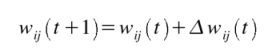
Stochastic minimization: This is the most trivial learning method. This is the Robbins-Monro stochastic approximation applied to multilayer perceptrons. The weights are updated after each example according to the formula:
with

The parameters for this method are Eta, EtaDecay, Delta and Epsilon.
Steepest descent with fixed step size (batch learning): It is the same as the stochastic minimization, but the weights are updated after considering all the examples, with the total derivative dEdw. The parameters for this method are Eta, EtaDecay, Delta and Epsilon.
Steepest descent algorithm: Weights are set to the minimum along the line defined by the gradient. The only parameter for this method is Tau. Lower tau = higher precision = slower search. A value Tau = 3 seems reasonable.
Conjugate gradients with the Polak-Ribiere updating formula: Weights are set to the minimum along the line defined by the conjugate gradient. Parameters are Tau and Reset, which defines the epochs where the direction is reset to the steepes descent.
Conjugate gradients with the Fletcher-Reeves updating formula: Weights are set to the minimum along the line defined by the conjugate gradient. Parameters are Tau and Reset, which defines the epochs where the direction is reset to the steepes descent.
Broyden, Fletcher, Goldfarb, Shanno (BFGS) method: Implies the computation of a NxN matrix computation, but seems more powerful at least for less than 300 weights. Parameters are Tau and Reset, which defines the epochs where the direction is reset to the steepes descent.
Defining datasets and the network structure
Neural network are build from a set of “samples”. A sample is a set of values defining the inputs and the corresponding output that the network should ideally provide. In root this is a TTree entry.
Several constructors are available:
TMultiLayerPerceptron
(const char* layout, TTree*
data = NULL, const
char* training = "Entry$%2==0",
const char* test =
"");
TMultiLayerPerceptron
(const char* layout, const
char* weight, TTree* data =
NULL, const
char* training = "Entry$%2==0",
const char* test =
"");
TMultiLayerPerceptron
(const char* layout, TTree*
data, TEventList* training,
TEventList*test);
TMultiLayerPerceptron
(const char* layout, const
char* weight, TTree* data,
TEventList* training, TEventList*
test);
The first thing to be decided is the network layout. This layout is described in a string where the layers are separated by semicolons. The input/output layers are defined by giving the expression for each neuron, separated by comas. Hidden layers are just described by the number of neurons. In addition, output layer formulas can be preceded by '@' (e.g "@out") if one wants to also normalize the output (by default, only input neurons are normalized). Expressions are evaluated as for TTree::Draw().
Input and outputs are taken from the TTree associated with the network. This TTree can be given as argument of the constructor or defined later with TMultiLayerPerceptron::setData().
Events can also be weighted, then the weight expression must be given in the constructor or set later with TMultiLayerPerceptron::setWeight().
Two datasets must be defined before learning the network: a training dataset which is used when minimizing the error, and a test dataset which will avoid bias. Those two datasets can be build aside and then given to the network, or can be build from a standard expression. By default, half of the events are put in both datasets.
Training the neural net
The learning method is defined using the TMultiLayerPerceptron::SetLearningMethod() . Learning methods are :
TMultiLayerPerceptron::kStochastic,
TMultiLayerPerceptron::kBatch,
TMultiLayerPerceptron::kSteepestDescent,
TMultiLayerPerceptron::kRibierePolak,
TMultiLayerPerceptron::kFletcherReeves,
TMultiLayerPerceptron::kBFGS
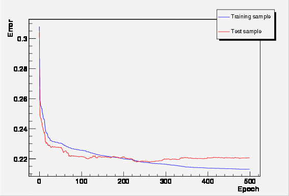
One starts the training with TMultiLayerPerceptron::Train(Int_t nepoch, Option_t* options). The first argument is the number of epochs while option is a string that can contain: "text" (simple text output) , "graph" (evoluting graphical training curves), "update=X" (step for the text/graph output update) or "+" (will skip the randomisation and start from the previous values). All combinations are available.
Example: net.Train(100,”text, graph, update=10,+”).
Controling and using the resulting network
Training a neural network is of course not a goal by itself. On needs after all to use it, look at the distribution, export it, etc. This is just an overview of all the possibilities. The detailled function prototypes are documented in the reference manual.
The DrawResult() method will produce an histogram with the output for the two datasets. The two arguments are the index of the output neuron desired and a string telling which dataset to use (“train” or “test”) and whether a X-Y comparison plot should be drawn (“comp”).
The weights can be saved to a file (DumpWeights) and then reloaded (LoadWeights) to a new compatible network.
The output can be evaluated (Evaluate) for a given output neuron and an array of double input parameters.
The network can be exported (Export) as a standalone code. Up to now this is only as a C++ class, but other languages could be implemented.
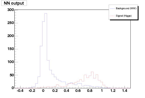
Separating signal Higgs events from background (WW) events
A nice example of how to use TMultiLayerPerceptron is part of ROOT tutorials: mlpHiggs.C
Using some standard simulated information that could have been obtained at LEP, a neural network is build which can make the difference between WW events and events containing a Higgs boson.
Starting with a TFile (mlpHiggs.root) containing two TTrees, one for the signal, the other for the background, a simple script is used. Those 2 trees are merged into one, with an additionnal type branch. The network that is then build has 4 input neurons, 8 additional ones in the only hidden layer and one single output neuron.
 |
 |
Fitting a magnetic field to import it into a simulation (G4) code
|
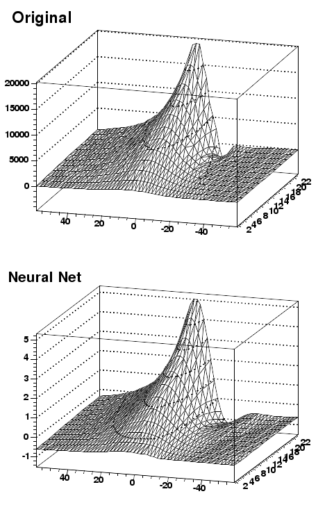
For some application with a cylindrical symmetry, a magnetic field simulation gives as output the following data:
One want to fit those distributions with a function in order to plug them into a Geant simulation code. On could try polynomial fits, but it seems difficult to reach the desired precision over the full range. One could also use a spline interpolation between known points. In all cases, the resulting field would not be C-infinite. A small compiled ROOT script was then used to fit those three distributions. This fitting procedure is lenghty compared with standard procedure, but do not need an a priori knowledge of the function behaviour. An example of output (for Br) is shown. First, the initial function that can be seen as the target. Then, the resulting (normalized) neural net output. In order to ease the learning, the "normalize output" was used here. The initial amplitude can be recovered by multiplying by the original standard deviation and then shifting by the original mean. The resulting exported functions are: |
 |
When you train your network in the Higgs example, you present all the signal events first and next the background events. I have seen in publications on neural networks that we must take care to present signal and backround events alternatively not to introduce bias in the learning. Is it true ?
Yes, to some extend.
For the stochastic minimisation, weights are updated after each event. There,
it's important to "shuffle" examples before training the network. This task
is carried on automatically.
For the 5 other methods, this is not needed since the global error is
computed, and the weights are updated after a loop on all events.
I haven't seen the normalisation of the inputs. Is it done automatically or we must call a function ?
It's automaticly done by the network. In the constructor of a input neuron, TTree::Draw() is used to extract the mean and the RMS of the corresponding variable. You'll see that normalisation explicitely in the function created by TMultiLayerPerceptron::Export().
My favorite question in not listed in the F.A.Q. . What can I do ?
Send it to the ROOT mailin list, or better post a subject to the ROOT forum. I'll be glad to answer it.
Theorem 1
K.Hornik et al., Multilayer Feedforward Networks are Universal Approximators, Neural Networks, Vol. 2, pp 359-366 (1989)
Theorem 2
D.W.Ruck et al., The Multilayer Perceptron as an Approximation to a Bayes Optimal Discriminant Function, IEEE Transactions on Neural Networks, Vol. 1, nr 4, pp296-298 (1990)
Stochastic minimisation
H.Robbins and S.Monro, A Stochastic Approximation Method, Annals of Math. Stat. 22 (1951), p. 400
S.E.Fahlman, An Empirical Study of Learning Speed in Back-Propagation Networks, CMU-CS-88-162 (1988)
Conjugate gradiant methods
R. Fletcher and C.M. Reeves "Function minimization by conjugategradients", Computer J. (1964) 149:154
E. Polak and G. Ribiere, "Note sur la convergence de methodes de directions conjuguees", Revue Francaise d'informatique et de recherche operationelle 16 (1969) 35:43
BFGS minimisation
C.G. Broyden "The convergence of a class of double-rank minimization algorithms", J. Inst. Math. Applcs. 6 (1970) 76:90
R. Fletcher, "A new approach to variable metric algorithms", Computer J. (1970) 13 (1970) 317:322
D. Goldfarb, "A family of variable metric methods derived by variational means", Math. Computation 24 (1970) 23:26
D.F. Shanno, "Conditioning of quasi-Neuwton methods for function minimization", Math. Computation 24 (1970) 647:657
TMultiLayerPerceptron is part of the ROOT distribution since ROOT 3.10/01 (added to the head end of August 2003). It's nevertheless still evoluting are lost of features were only added to ROOT 3.10/02.
C. Delaere - January 2004