SiStrip Simulation overview
Special meeting 13-05-2014
Claude Nuttens (claude.nuttens@cern.ch)


Table of Contents
Outline
- Links & docs
- The job
- SiStrip Digitization steps overview
- SiStrip Digitizer software structure
- The first project
- Some Details on modules
Links & doc
- Your future kingdom the « SiStripDigitizer »: github and lxr links
- Tracker DPG
- hypernews: hn-cms-trackerperformance@cern.ch
- indico
- Offline sim:
- hypernews: hn-cms-simDevelopment@cern.ch
- indico
- CMSSW releases schedule
- Subscribe to relval hn-cms-relval@cern.ch
- My personnal documentation: personnal link
- SiStrip Simulation, LocalReconstruction and Calibration page: Twiki page
- SiStripDigitization wiki: Twiki page
- This presentation: link (classic slides here)
The Strip Sim contact Job
- Be aware of what happened to the SiStripDigitizer
- Be aware on things that could touch the sim in Strip
- Be the interface between the offline sim group and the Tracker group
- Answer (physics/performance) improvement requests, bugs, ... and implement it if needed
- Keep an eye on the Relval on MC (not your job but check the status report)
Strip Digitizer Structure ↓
From Geant 4
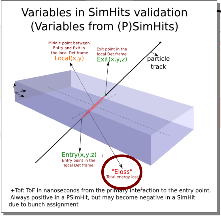
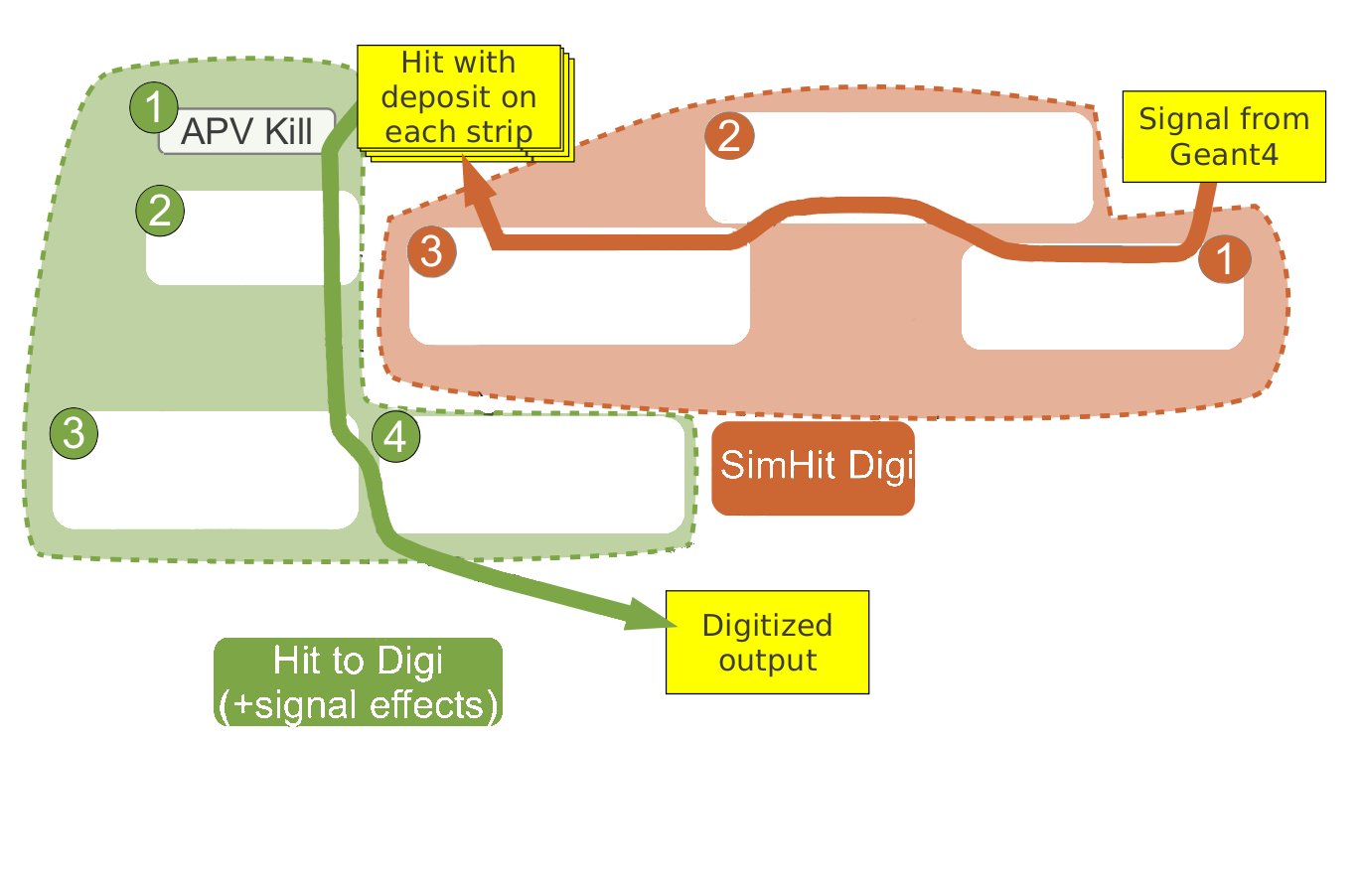
Strip signal simulation steps

Sim Hit deposit simulation
‹ ›
›
- "Divide deposit" and "Crosstalk" in previous slide step-picture
- be carefull! scales, strip density, ... are not trustfull, some effects are exaggerated for the representation/understanding (also to be check strip orientation in the local reference frame, x or y?)
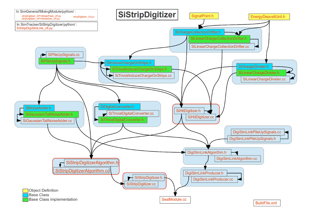
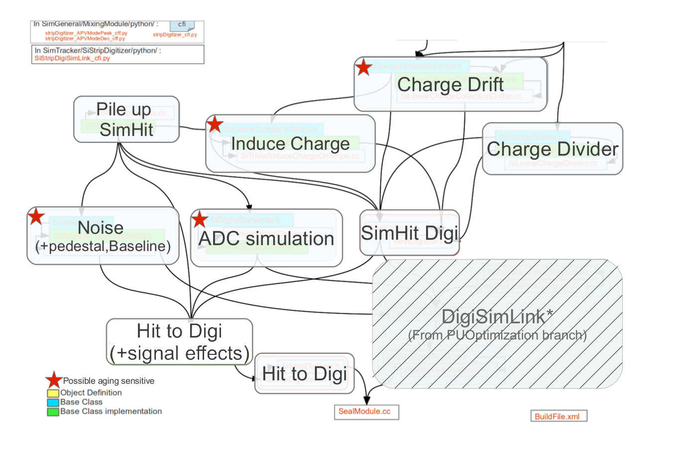
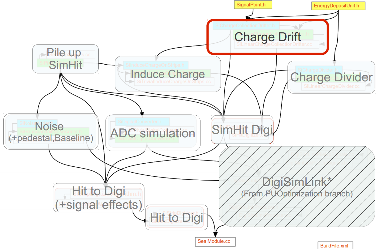
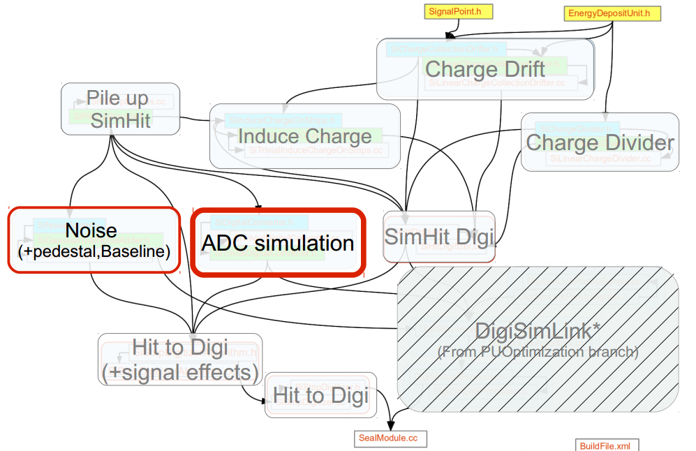
SiStrip Digitizer structure
| Detailled view | Module view | Time View |
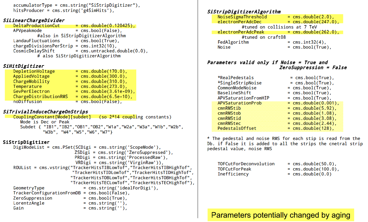
StripDigitizer parameters
In /SimGeneral/MixingModule/python/stripDigitizer_cfi.py
First Project ↓
Impact of the Temp. param.
- Study the impact of the Temperature parameter on the simulation
Seen in previous slide :
Temperature = cms.double(273.0), - This parameter is used in the diffusion constant computation
required to compute the drift time of the charge in the sensor
(we will see a bit further)
→ As seen before, the charge drift is one of the first step - In 2015 runs, the temperature is lowered to ~-20°C,
- How does distributions are impacted by this change?
- If you see impact, how a few degrees variations around this value
impact the distributions
→ to see if keeping a global temperature is a fair approximation
- Note that it may not be the only temperature effect in the simulation,
as other parameters used/defined are temperature dependent but
not defined from this configuration temperature value.
You can try to list temperature dependence in the sim.
(not mandatory, we can see together when you have the first results)
Details of modules ↓
Depletion and applied voltage
Depletion and applied voltage
- In
SiHitDigitizer.cc:double timeNormalisation = (moduleThickness*moduleThickness)/(2.*depletionVoltage*chargeMobility);
$ t_{Norm} = \frac{Thickness_{mod}^2}{2. V_{Depl}. chargeMobility}$ where $ chargeMobility \propto \left[ \frac{cm^2}{V.s} \right] $ - In
SiLinearChargeCollectionDrifter(drift time in the sensor)double driftTime = -timeNormalisation *log(1.-2*depletionVoltage*thicknessFraction/(depletionVoltage+appliedVoltage)) +chargeDistributionRMS
SignalPoint drift (EnergyDepositUnit edu, Localvector drift, moduleThickness, timeNormalisation)see next slide - This have an effect on coupling wich use the chargeSpread
Depletion and applied voltage
SignalPoint drift (EnergyDepositUnit edu, Localvector drift, moduleThickness, timeNormalisation)
- computes the fraction of the module the charge has to drift through,
$ depth=\frac{moduleThickness} {2}- energyDeposit.z()$
$ thicknesFraction=\frac{depth}{moduleThickness}$ - ensure thicknessFraction $\in [0,1]$
- Compute the drift time in the sensor
$ driftTime = −t_{Norm}∗log \left(1−\frac{2.V_{Depl}}{V_{Depl.}+V_{Appl.}}\cdot thicknessFraction \right) +chargeDistributionRMS $ - Return the SignalPoint(x,y,sigma,amplitude): pos., an energy on the surface, with a size due to diffusion.
$SignalPoint(edu.x ()+\frac{depth∗drift.x ()}{drift.z()}, edu.y ()+\frac{depth∗drift.y()}{drift.z()},\sqrt{2.∗diffusionConstant∗driftTime} , edu.energy ())$ where
$diffusionConstant= \frac{CBOLTZ}{e}∗chargeMobility∗Temp∗{1.0 if noDiffusion \choose 1.0e-3! noDiffusion}$
Noises, pedestal and baseline

Noises in Zero suppression

Noise in Zero suppression
- Produce noise using GaussianTailNoiseGenerator
- Gaussian Noise on strips with signal with CLHEP::RandGaussQ(rndEngine):
- Loop on channels and add noise if not null in[iChannel] += gaussDistribution->fire(0.,noiseRMS);
- Noise on the other strips
- Loop on generatedNoise vector pair generated at top
- Add to channel the corresponding noise (and check that value ==0) in[(*p).first] += (*p).second;
- Loop on generatedNoise vector pair generated at top
Gains
Couplings
